
Start with a picture
A handwritten digit is a useful first input to a neural network. You can see the shape, understand the task, and recognise a mistake. It also gives us a concrete way to explore a less familiar question:
What happens when a network learns through the timing of spikes?
In this walkthrough, we use Next Brain's Training Studio to train a small spiking neural network on MNIST. We follow the path from pixels to activity, inspect the connections that change, evaluate the frozen network on separate images, and save a model for inference.
The example is deliberately small. Its purpose is to make a complete learning experiment understandable and repeatable. The measurements below come from a real run of the platform's trusted training adapter through the Brian2 Atlas CPU engine; they are not interface demonstration data.
From pixels to a prediction
MNIST contains 28 × 28 grayscale images of handwritten digits. Its published pools contain 60,000 training and 10,000 test images; this tutorial uses small, explicitly selected subsets. MNIST dataset source.
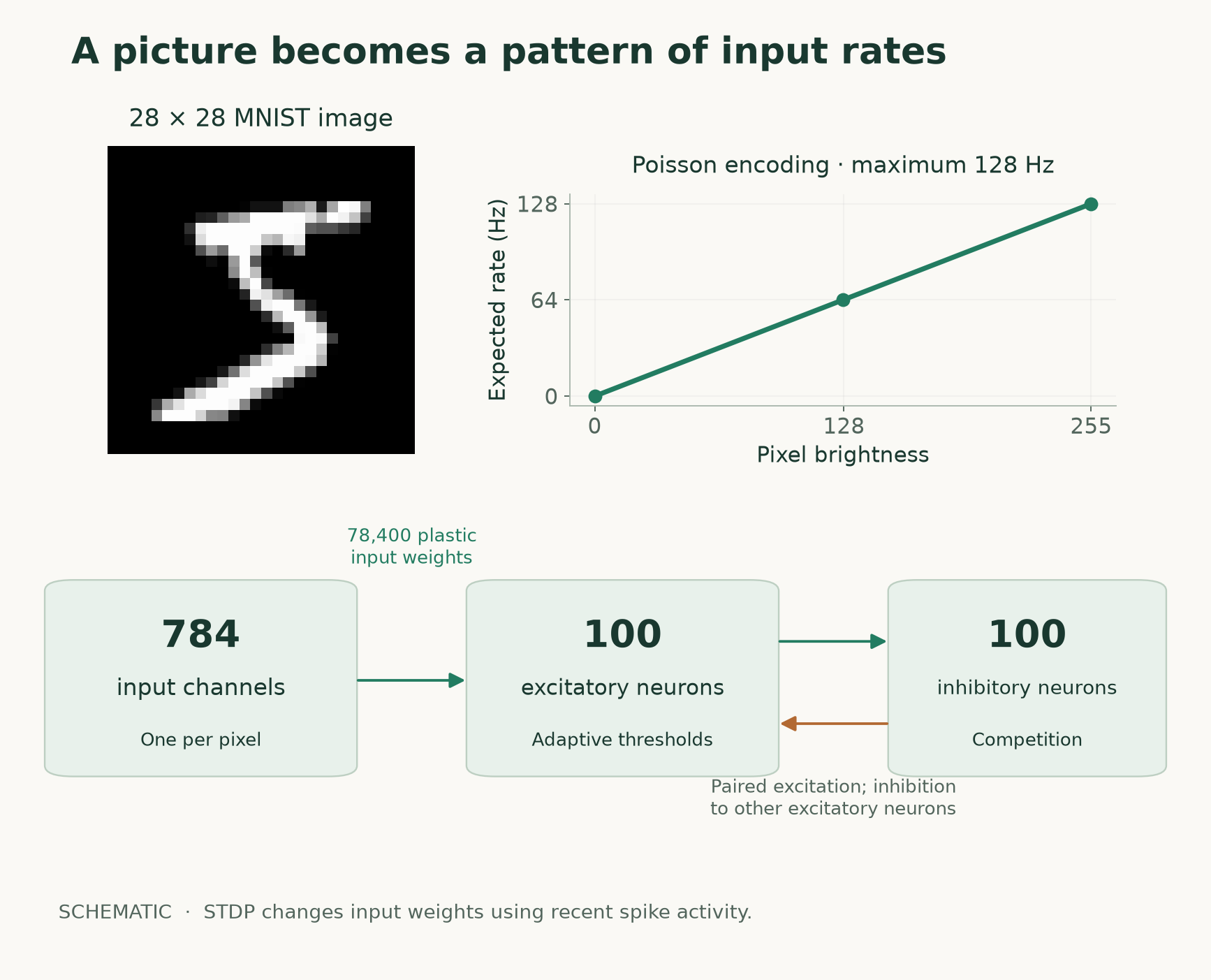
Figure 1. Input and network schematic. Pixel brightness controls an expected input firing rate. The diagram explains the configured mechanism; it is not a recording of spike times.
There are 784 input channels, one for each pixel. With Poisson rate encoding, a brighter pixel produces a higher expected rate of input spikes. At our chosen maximum rate of 128 Hz, a black pixel has a rate of zero and a fully bright pixel has an expected rate of 128 Hz. Individual spike times are random.
Those inputs connect to 100 excitatory neurons through 78,400 adjustable weights. A paired population of 100 inhibitory neurons creates competition: excitation recruits inhibition that acts on other excitatory neurons. Adaptive thresholds also change during learning.
The learning rule is triplet spike-timing-dependent plasticity, or STDP. It updates an input connection using traces of recent presynaptic and postsynaptic spikes. Repeated input and response patterns can therefore change which inputs drive each neuron. Weight normalisation helps control the scale of those connections.
The platform adapts the Brian2 Diehl–Cook example, based on Diehl and Cook's 2015 study. Our compact network, small data budget and fixed-duration presentations are a teaching configuration, not a reproduction of the paper's reported accuracy.
Where do the digit labels enter?
The synaptic learning rule does not use digit labels. A neuron also does not inherently know that its activity means “7.”
After freezing learning, the platform presents a separate class-assignment set. It uses the labels of those images to determine which digit class each neuron responds to most strongly on average. For prediction, it compares average spike counts across the assigned neuron groups.
This distinction matters: the weights learn without labels, while the classification readout uses labels. Validation scoring and final testing use other images.
Configure a small teaching run
Open Training Studio and sign in with an account that has access. If registration is currently invitation-only, use your invitation or join the waitlist. Execution also requires an available training worker.
The setup has four screens: Model, Dataset, Protocol and Review.
On Model, select Compact STDP and retain 784 model inputs. The compact option has 100 excitatory neurons and 100 inhibitory neurons, in addition to the input channels.
On Dataset, select MNIST and click Prepare MNIST if it is not ready. Preparation downloads or reuses the source files, verifies them and audits the inputs. Keep the native 28 × 28 grayscale shape and select Poisson rate encoding.
Use the following settings for this walkthrough. These override the larger default sample counts and five-epoch default.
| Setting | Tutorial value |
|---|---|
| Model | Compact STDP: 100 excitatory + 100 inhibitory neurons |
| Input | MNIST, native shape, 784 inputs |
| Training images | 200 |
| Validation images | 100, divided into 50 class-assignment and 50 scoring images |
| Test images | 100 from the official test pool |
| Epochs | 1 |
| Starting seed | 42 |
| Encoding | Poisson, maximum input rate 128 Hz |
| Each presentation | 350 ms stimulus + 150 ms rest |
| Sample order | Shuffled |
| Between samples | Continuous dynamics with a rest period |
| Automatic checkpoint | Every epoch |
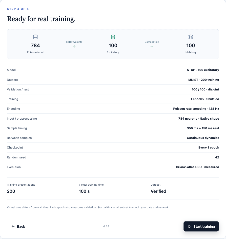
Figure 2. The Review screen brings the network, data budgets and learning protocol together before you submit a job. This screenshot uses the tutorial settings.
An epoch is one pass through the selected training images. One epoch here means 200 training presentations. Those presentations cover 100 seconds of simulated time. Baseline measurement, class assignment, validation and testing add more simulation; none of these durations is a promise about wall-clock waiting time.
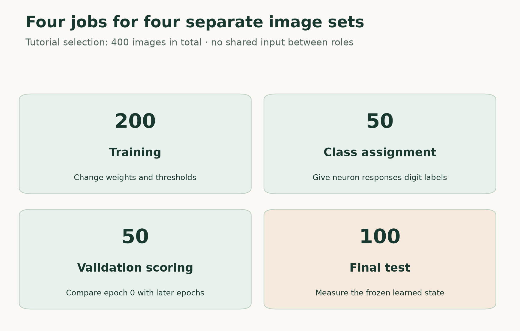
Figure 3. The 100-image validation budget serves two separate roles. Class assignment establishes the readout; validation scoring measures it on other images. The same selected IDs are reused across epochs.
The platform saves the concrete sample selections and checks for input overlap. For this MNIST example, training and validation come from the official training pool, while testing uses the official test pool. If you later upload related recordings, provide participant or session groups so related samples stay together.
Review the configuration, then click Start training. The job runs on the server's CPU worker. Its progress and checkpoints persist independently of the browser page. You can pause at a sample boundary and resume from verified state when the required runtime is available.
Compare the network before and after training
The Overview tab brings together progress, measured validation scores and, after training completes, learned input weights. With our one-epoch setting, the curve has a starting point and one completed post-training point.
Start with epoch 0. Before STDP training, the platform freezes the random initial network, assigns neuron classes and measures validation accuracy. The post-training measurement uses the same assignment and scoring images after the single training epoch.
The dotted 10% line represents uniform guessing among ten labels. The epoch-0 point is different: a measured random network with a calibrated readout. It can perform above or below 10%. To assess what training changed in this run, compare the post-training validation point with that measured starting point.
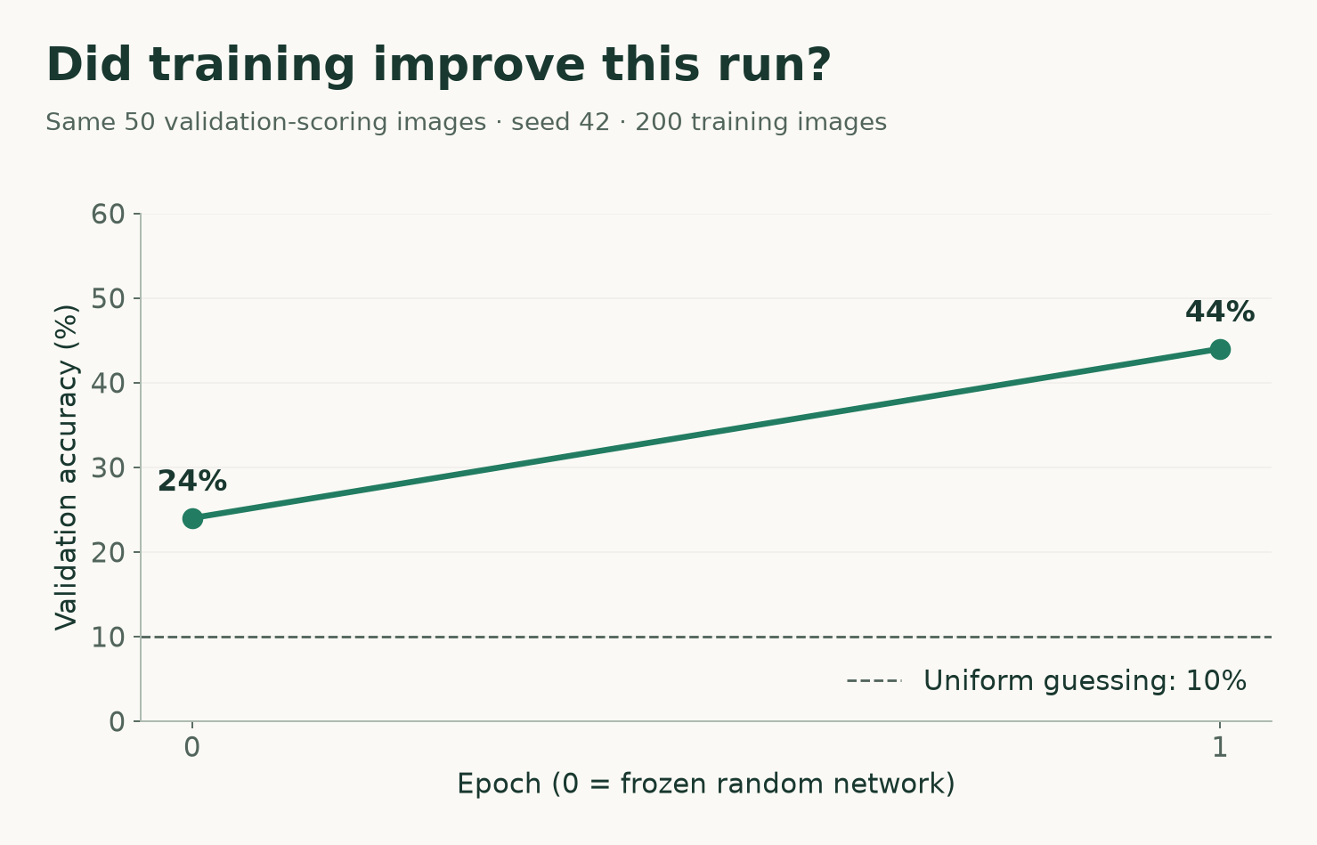
Figure 4. Two measured states of the same tutorial network. Both points use the same 50 class-assignment images and a separate fixed set of 50 validation-scoring images.
In this run, validation accuracy changed from 24% before training to 44% after one epoch: 12 correct predictions out of 50 became 22 out of 50. That is a 20-percentage-point increase under this training procedure, which includes weight changes, adaptive thresholds and readout recalibration.
This comparison describes one small run. It does not isolate the contribution of each mechanism; that would require further controls.
A learning curve need not rise smoothly. A small scoring set is noisy, and improving a training objective does not guarantee better classification. This walkthrough uses one seed and a small subset; it does not estimate performance across seeds or establish a general accuracy claim.
Look at the connections
Each excitatory neuron has 784 input weights. Reshaping them into a 28 × 28 image makes its input preferences visible. Brighter positions represent stronger connections from those pixels.
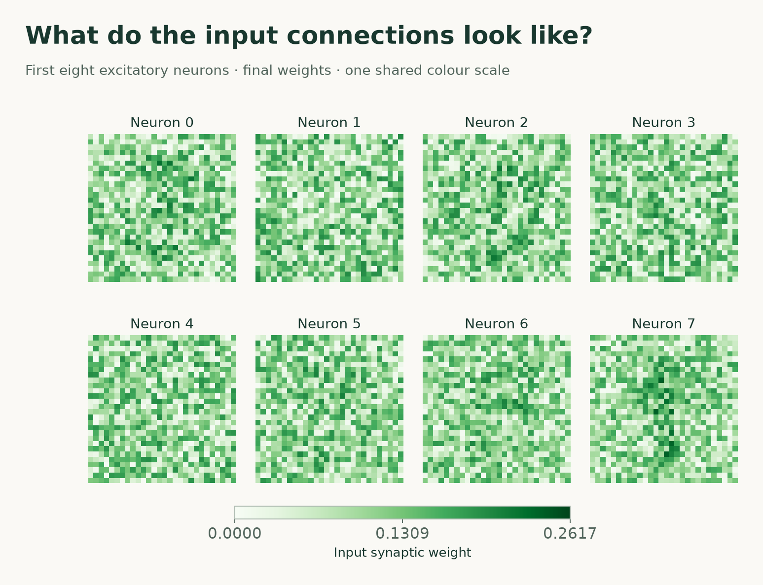
Figure 5. The first eight neuron fields after one training epoch, shown with a shared colour scale from zero to the recorded maximum weight. These are the recorded weights, without selecting fields for how much they resemble digits.
At this early stage, the displayed fields remain diffuse; they do not yet form clear digit templates. That is worth keeping beside the improved validation score.
Training Studio displays eight measured neuron fields. They are a view into the learned state, not reconstructed input images or proof that every neuron represents a distinct digit. For MNIST, all 784 weights of each displayed neuron fit in the view; larger inputs use sampled features.
Test the frozen model, then use it
Open Evaluation and click Run evaluation. The platform freezes both synaptic plasticity and adaptive thresholds and evaluates the separate test images.
Read the confusion matrix as well as the overall score. Rows are true labels; columns are predicted labels. The diagonal counts correct predictions. Off-diagonal cells reveal specific confusions. The “No response” column counts cases with no assigned response, and those cases remain in the accuracy denominator.
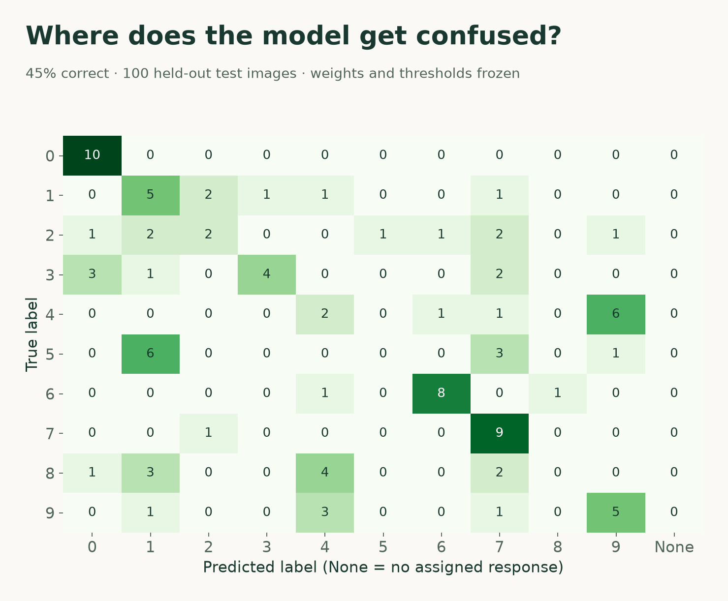
Figure 6. The model classified 45 of 100 test images correctly (45%). Each true digit has ten test examples. All produced an assigned response, so there were no abstentions.
The overall score hides substantial differences between digits: all ten zeros were classified correctly, but none of the ten examples for either digit 5 or digit 8 were correct. In this sample, six fours were classified as nines. Those are concrete places to investigate before treating the model as a useful digit recogniser.
The interface also distinguishes genuinely silent samples from samples that produced spikes only in unassigned neurons. A missing class assignment is a useful diagnostic: activity alone does not guarantee that the readout can represent every digit.
After evaluation, open Trained model, give the model a name and click Save trained model. Then select Load for inference, choose one of the supplied test-set examples and click Run inference. The current interface loads the sample as input JSON; you can also provide another input in the original dataset format.
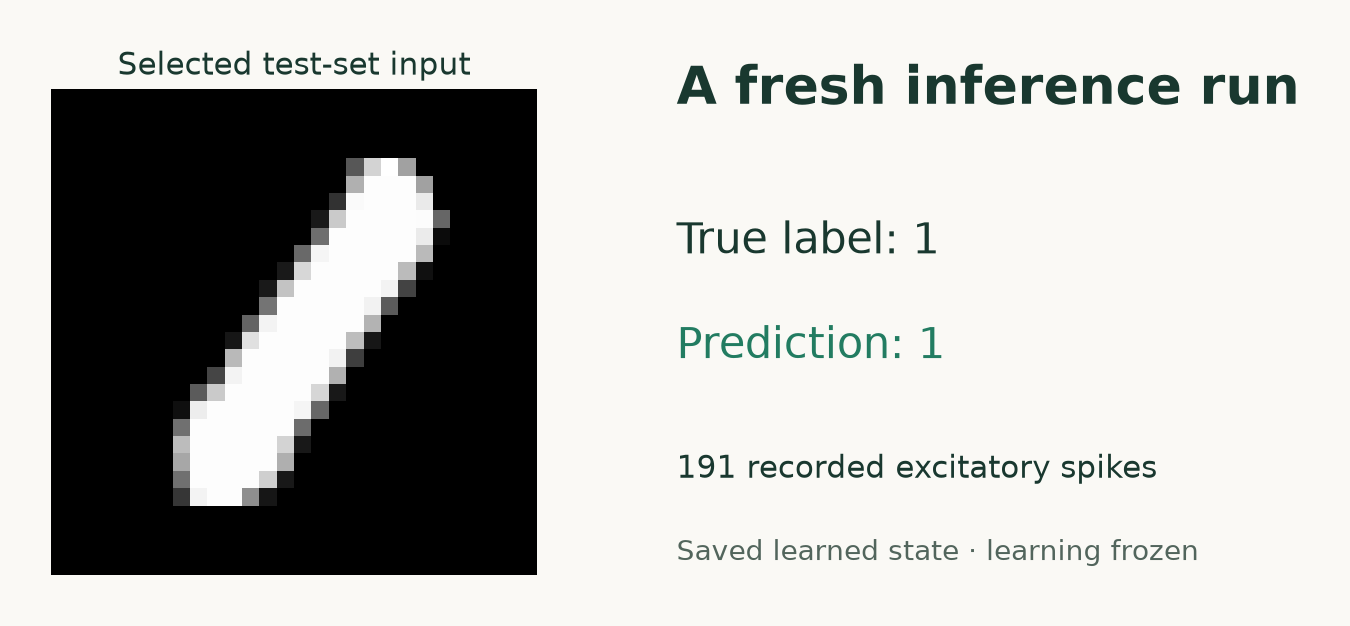
Figure 7. We used the first test example returned by the platform: platform sample 67900, true label 1. The saved model predicted 1 and produced 191 recorded excitatory spikes. This prediction is correct.
Inference starts a fresh network with the saved learned state and learning frozen. It is a new numerical execution. A single example is useful for checking the workflow, but its prediction is not an additional accuracy benchmark and can differ from a prediction made inside a continuous evaluation sequence.
Download learned model exports the learned arrays, a manifest, the exact trusted trainer source and a readme. The arrays include weights, adaptive thresholds and neuron-class assignments. The export does not contain the dataset or a self-contained executable runtime.
What the platform takes care of
A small experiment still involves many pieces: preparing inputs, keeping evaluation separate, running the simulator, preserving state and connecting a score to the configuration that produced it.
Training Studio keeps those pieces together. Each submission snapshots the dataset metadata, configuration and trainer source version. The selected sample roles are recorded. Checkpoints retain network and random state, and the account history gives you a way back to previous training jobs. The measured curves, weight views and evaluation all belong to that saved job.
This makes it easier to ask the next question without losing the history of the first one. You still decide which comparison is meaningful, whether the sample size is adequate and what the evidence supports.
Three useful next experiments
Give the network more training data. Keep the architecture and encoding fixed, choose a larger training subset and compare validation behaviour. Decide the comparison before repeatedly inspecting final test scores. More presentations alone do not guarantee better results.
Change the input domain. Fashion-MNIST offers another 28 × 28 image task through the same dataset workflow. Training Studio also accepts validated user CSV or JSON inputs, including feature vectors and spike events. Different data require appropriate input dimensions, encoding and split design; a supported format does not guarantee a useful classifier.
Compare encoding intensity systematically. Once a single training run is familiar, open Experiments and choose Learning & plasticity. That workflow runs the prepared dataset under several Poisson encoding intensities, repeats conditions and compares measured held-out accuracy. Its current comparison keeps STDP enabled; it does not switch between arbitrary learning rules.
The current Training Studio uses a defined STDP architecture through the Brian2 Atlas CPU path. It is suited to exploring local plasticity, inspecting learned connections and carrying a trained state through evaluation to inference. Arbitrary model training, gradient backpropagation and GPU training are outside this adapter's present scope.
Start your first training run, follow the measured evidence, and keep the first question small enough that you can explain every part of the answer.
Sources and tutorial evidence
- MNIST source files and dataset description.
- Diehl, P. U. and Cook, M. (2015), Unsupervised learning of digit recognition using spike-timing-dependent plasticity.
- Brian2's Diehl–Cook example, the upstream example adapted by the platform.
- Download the tutorial measurements and provenance (JSON): configuration, selected sample IDs, baseline and final metrics, weight fields, inference input/output and recorded runtime fingerprints.
Authoring note: we initially planned three epochs, then reduced the tutorial to one for the local compute budget before inspecting any test result. We reused the verified first-epoch checkpoint, its exact data splits and the original baseline, and completed validation and testing in a one-epoch job. The parent run and preparation note are recorded in the evidence file. Readers can select one epoch from the outset; the ordinary setup above does not require this author-side preparation step.